Modeling Background Radiation with Hidden Markov Model

Introduction

This project studies the problem of estimating environment gamma-ray radiation with Hidden Markov Model (HMM). Environment radiation major comes from natural radioactive materials in the environment, such as potassium-40, thorium-232 and uranium-238 in the soil and radon-226 in the air. Studies have shown that the concentration of radioactive materials in the environment can be affected by precipitation, and the background radiation thus will fluctuate as weather condition changes. This project aims at modeling the fluctuation behavior of background radiation based on radiation measurements using HMM. Because decay events from radioactive materials follow Poisson distribution, the Poisson Hidden Markov Model is used.

Experiment Design

In this project, both radiation measurements and precipitation measurements were required. We deployed a small weather station together with a scintillator gamma-ray detector to collect radiation and precipitation data for a period of seven days. The radiation measurements recorded the gamma-ray count rate in every second, and the weather station recorded the precipitation information in every 10 minutes.

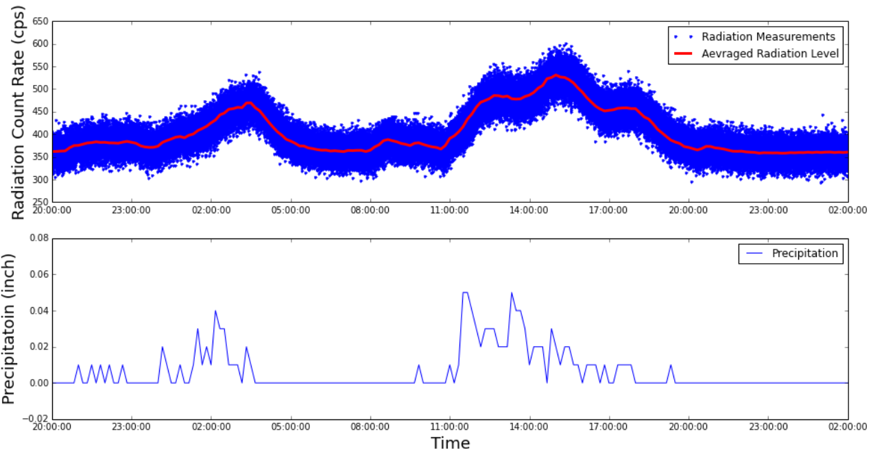
Figure 1. Recorded background radiation and precipitation measurements between 2016-11-27 20:00 and 2016-11-29 2:00

Figure 1 shows that the background radiation level changed from hours to hours. However, in the time interval of ten minutes the background radiation level could be considered as constant. For each ten minutes, the average count rate was calculated and treated as the ground truth radiation level for that time interval. According to the Poisson distribution, the more measurements are acquired, the better estimation can be calculated. For the ground truth radiation level, each mean value was estimated by 600 measurements (1 seconds * 600 = 10 minutes). The question is whether this radiation ground truth value can be estimated accurately with fewer measurements. In this project, we used a Poisson Hidden Markov Model to approximate this ground truth radiation level with much less measurements in each time interval.

Poisson Hidden Markov Model

In our project, the background radiation was modeled by Poisson Hidden Markov Model (PHMM). The background radiation levels were treated as hidden states, which formed an unobservable discrete time Markov Chain. The step size for time was 10 minutes. Each hidden state corresponded to a Poisson distribution which generated the radiation measurements within the hidden state's time interval. This project was implemented by ghmm Python package, which doesn't support using Poisson distribution for emission probabilities. Gaussian distributions were used instead to approximate the Poisson distributions .

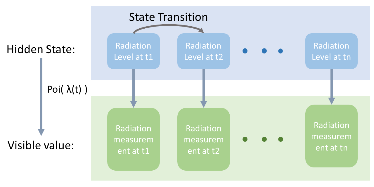
Figure 2. Illustration of Hidden Markov Model

Training:

There were in total 180 time-intervals in the dataset. Each time interval contained 600 measurements. Each measurement lasted for one second. For each time-interval, a measurement was randomly selected to form the training dataset, which had 180 one-second measurements in total. This training dataset was used to obtain the transition probability matrix and emission probability functions of the hidden Markov model, through the Baum-Welch algorithm implemented by ghmm package in python.

Prediction:

The same training dataset was used to predict the hidden state (radiation level) for 180 time-intervals based on the transition probability matrix and emission probability functions obtained in the training step, through the Viterbi algorithm implemented by ghmm package in python.

Results discussion

In the following three figures, HMM predictions (green line) were compared with the reference value of background radiation level (red line). All of the three HMM (3, 5, and 10 hidden states) captured the overall trend of background radiation. However, the HMM with 3 hidden states had too few hidden states to capture details of the change of background radiation. On the contrary, the HMM with 10 hidden states had too many hidden states that its prediction was too noisy and over-fitting to the measurements. The HMM with 5 hidden states provided the highest quality of prediction, and matched the reference level the best.

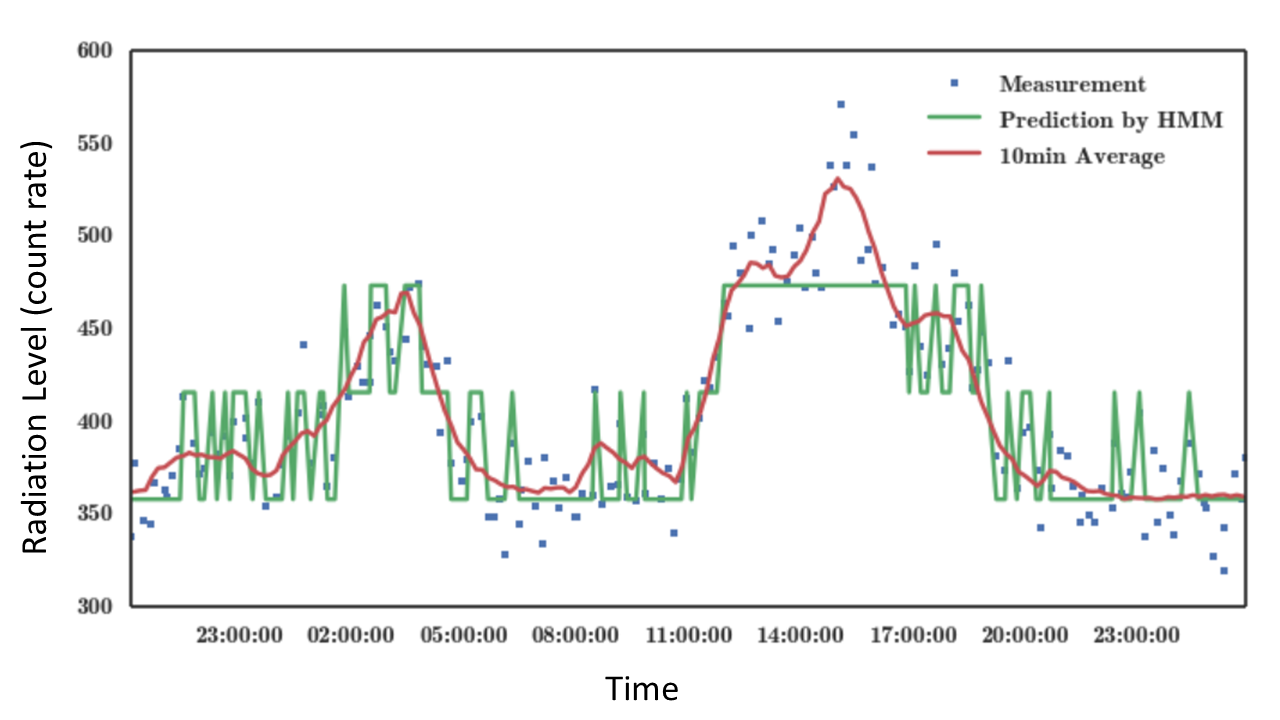
Figure 3. Prediction from 3 hidden state HMM.

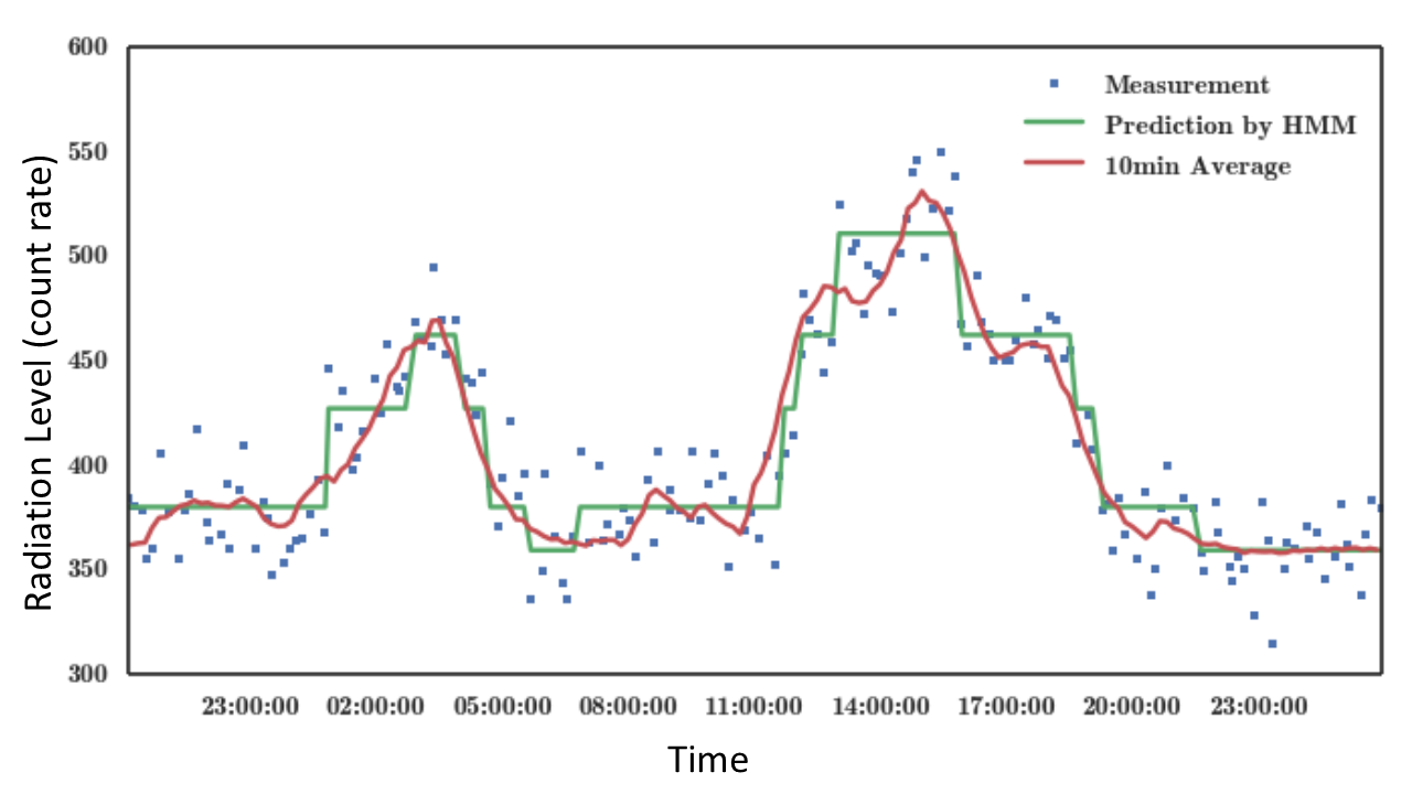
Figure 4. Prediction from 5 hidden state HMM.

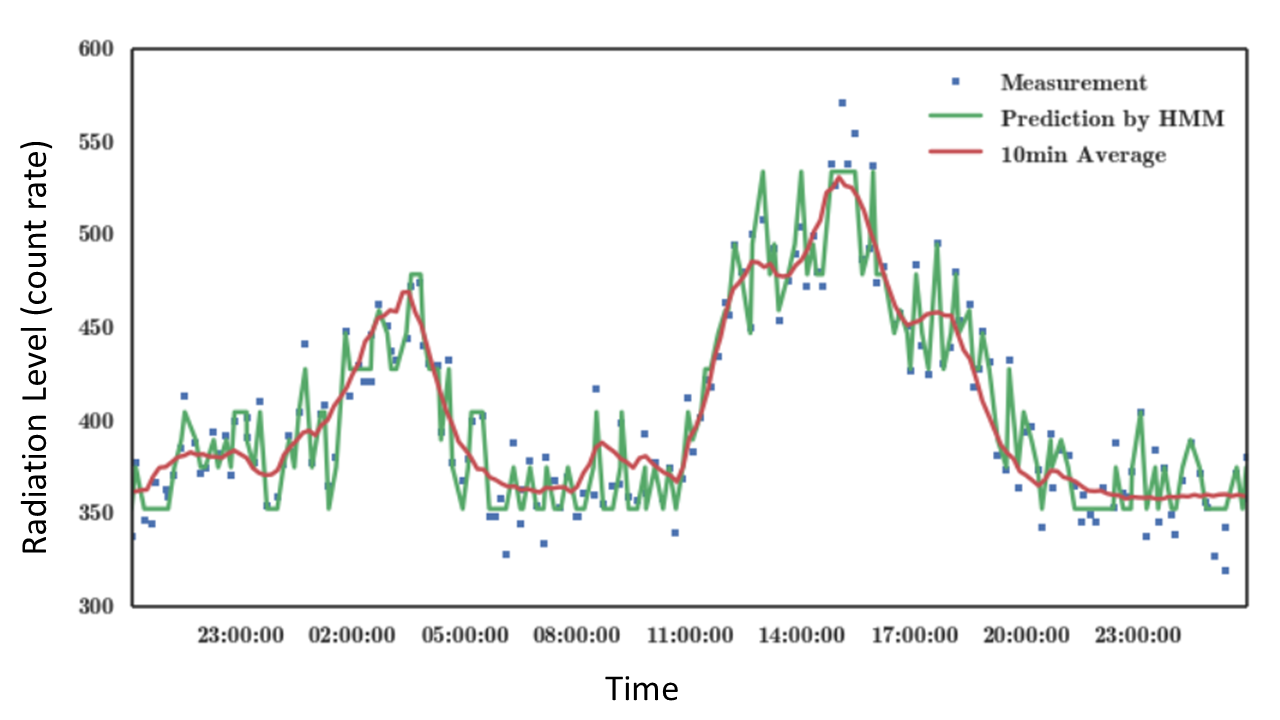
Figure 5. Prediction from 10 hidden state HMM.

Reference

[1]. Shahbazi-Gahrouei D, Gholami M, Setayandeh S. A review on natural background radiation. Advanced Biomedical Research. 2013;2:65. doi:10.4103/2277-9175.115821.
This paper explained the basic concepts and knowledge about background radiation, and discusseed different sources of background radiation in our daily life. This paper introduced my project’s background knowledge of radiation.

[2]. N. Salikhov and O. Kryakunova, “An increase of the soft gamma-ray background by precipitations,” International Cosmic Ray Conference, vol. 11, p. 367, 2011.
This paper discussed the correlation between precipitation and soft gamma-ray background radiation based on an experiment in Tien-Shan mountains. Their results showed that the environmental gamma-radiation background increased during precipitation.

[3]. "Markov Chains" by J. R. Norris First three chapter, especially section 2.4: Poisson Process.
This section describes the definition and properties of Poisson Process, which will be used to model the background radiation events.

[4]. Scott, Steven L. "Bayesian methods for hidden Markov models." Journal of the American Statistical Association (2011).
Demonstrated how to use recursive algorithms to simulate the parameters of Hidden Markov Model based on observed data.

[5]. GHMM Library homepage: http://ghmm.sourceforge.net/
This is the hidden Markov model package implemented in this project